

The more formulas you know how to use in Google Sheets, the better. For example, you never know when you’ll need to translate something to another language, so by learning how to do that now, you won’t waste time learning later. The good news is that the formula is easy to follow, and even if you’re in a hurry, it’s something you can do.
Contents
How to Use the Google Translate Formula in Sheets
When entering the formula, there are three things you need to keep in mind. You’ll need to add the cell that you want to translate. Then you’ll need to add the source language, followed by the target language. For example, if in Cell A1 you added the text: How are you? And you want Google Sheets to translate that to Spanish. To have the text translated, you’ll need to start typing =GOOGLETRANSLATE. As soon as you type the first few letters, the formula will appear, and you’ll need to click on it.
Once you’ve entered the formula, ensure it has an opening parenthesis, followed by the cell with the text you want to translate. You can enter the cell manually, or you can click on the cell. Make sure that the commas and quotes are placed in the correct places. Please look at the image below to see where they are placed. Once you’ve checked everything is where it should be, press enter, and your text should be translated automatically.
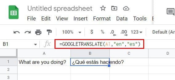
If you want to refresh your memory with how the formula is laid out, click on the cell where the translated text is. At the top, you should see the formula. You can also see more information explaining the formula if you click on it.

In the above formula, Google Sheets translated English to Spanish. But let’s see how you can make the formula auto-configurable. Remember that you can add the formula by going to the Insert tab at the top > Function > Google > Google Translate.

How to Apply the Formula to Other Cells Instantly
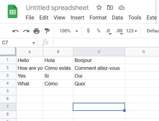
Let’s say you have other cells to which you want to apply the same formula. Don’t worry; you don’t have to copy and paste the formula to every cell. You have text in Spanish and English on your Google Sheets file, and you want to translate it to French. Once you have entered the text, you want to translate it into French (using French as an example); select the cell where you have the formula that translated the first phrase to French and drag it so that the cells below it are selected. As soon as you let go, all the empty cells will be filled with the translated text.
There is another language you can use to identify a language. On an empty cell, start typing =DETECTLANGUAGE. When the option appears, click on it and then click on the cell that has the language you want to identify. On the cell you entered, the formula will be replaced with the initials of the language.
Conclusion
There are so many languages out there that, sooner or later, you will need help identifying them. Thanks to a Google Sheets formula, you can identify them quickly. Also, applying the formula to every cell you want to translate is unnecessary. Even if you’re new to Google Sheets, using the Google Translate formula is an easy task. How many languages are you adding to your Google Sheets file? Share your thoughts in the comments below, and don’t forget to share the article with others on social media.


How do you disable Google incognito mode